Tutorial
Assuming you have the code setup it’s time to see what it can do. Fire up an interactive python session such as ipython and import splitwavepy as sw.
import splitwavepy as sw
Synthetic data
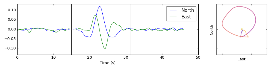
By default, if no data are provided, SplitWavePy will make some synthetic data. Data is stored in a Pair object. I will use synthetic data to demonstrate the basic features of the code.
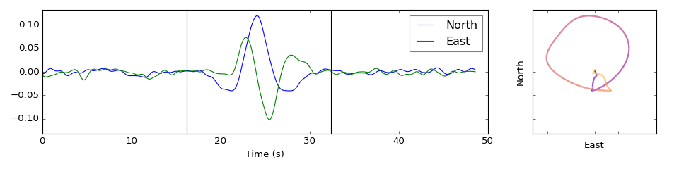
data = sw.Pair( split=( 30, 1.4), noise=0.03, pol=-15.8, delta=0.05)
data.plot()

You can simulate splitting by specifying the fast direction and lag time using the split = (fast, lag) argument, similarly you can specify the noise level, and source pol -arisation as shown in the example above. Order is not important.
Note
Don’t forget to set the sample interval delta appropriately (defaults to 1), it determines how your lag time is interpreted.
Adding and removing splitting
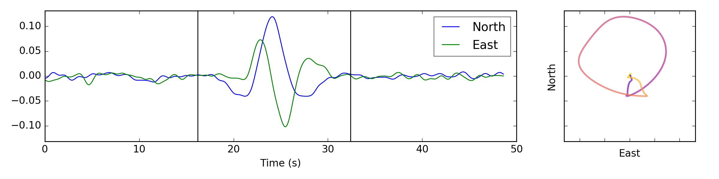
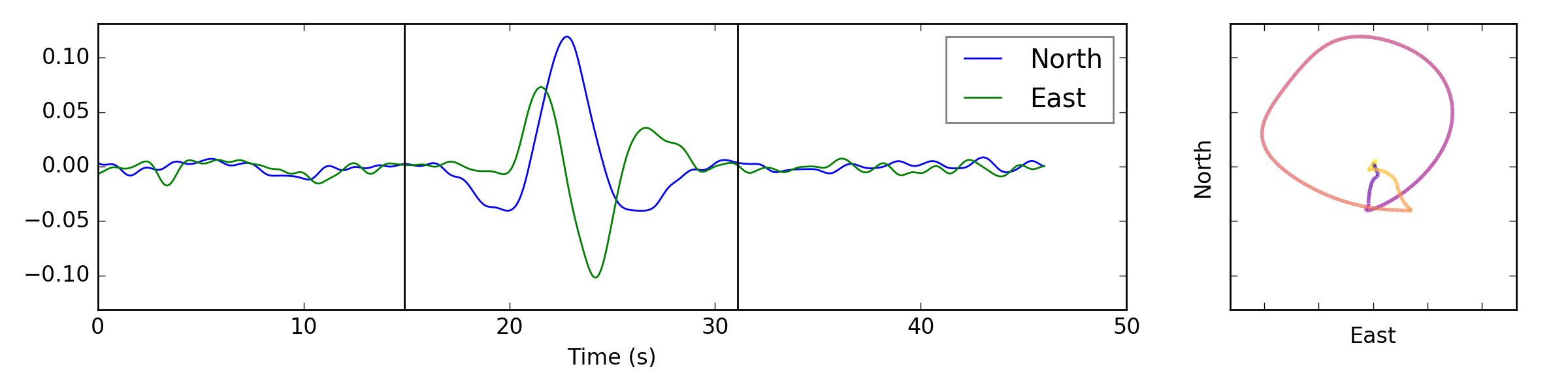
The data are already split, but that doesn’t mean they can’t be split again! You can add splitting using the split() method.
data.split( -12, 1.3) # fast, lag
data.plot()
Note
This method will also split the noise, which is probable undesirable. A better way to make synthetic with multiple splitting events is to provide the split keyword with a list of parameters, e.g. split = [( 30, 1.4), ( -12, 1.3)], these will be applied in the order provided.
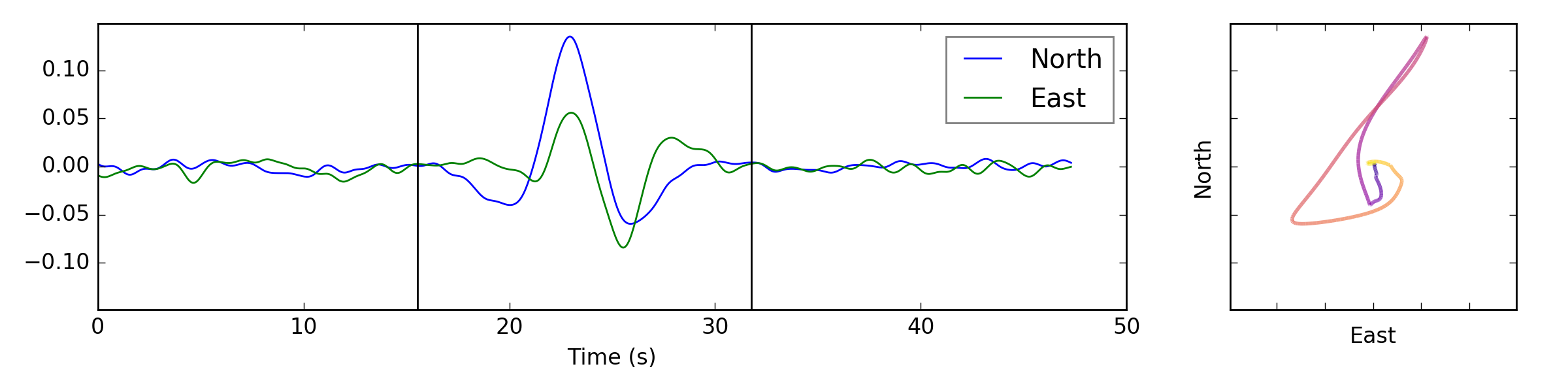
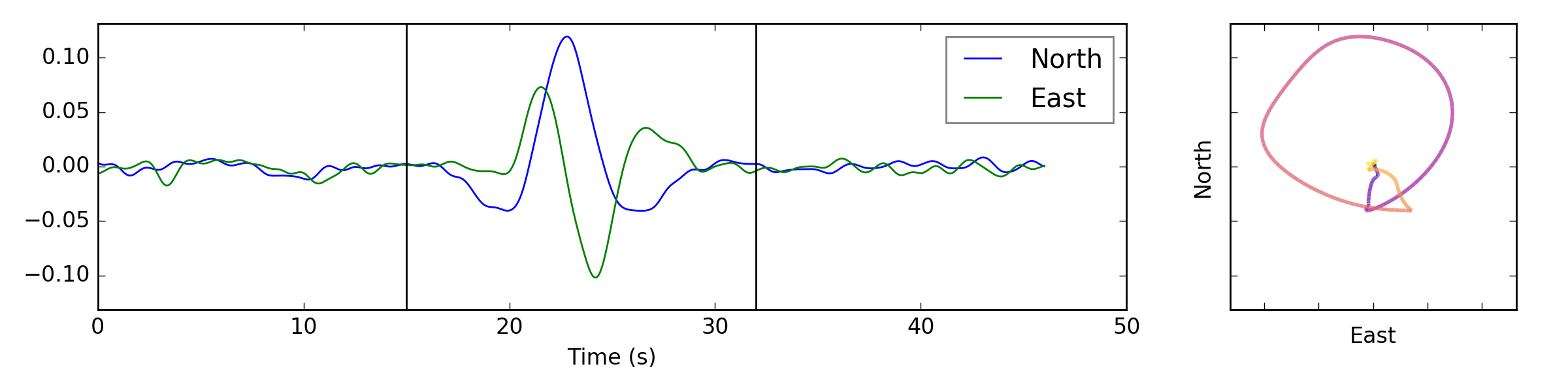
Sometimes we might want to do a correction and apply the inverse splitting operator. This is supported using the unsplit() method. If we correct the above data for the latter layer of anisotropy we should return the waveforms to their former state.
data.unsplit( -12, 1.3)
data.plot()

Note
Every time a lag operation is applied the traces are shortened. This is fine so long as your traces extend far enough beyond your window.
Setting the window
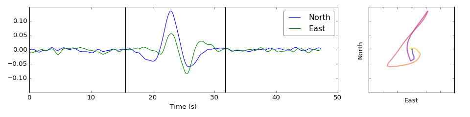
The window should be designed in such a way as to maximise the energy of a single pulse of shear energy relative to noise and other arrivals.
Set the window using the set_window(start,end) method.
data.set_window( 15, 32) # start, end
data.plot()

Note
By default the window will be centred on the middle of the trace with width 1/3 of the trace length, which is likely to be inappropriate, so make sure to set your window sensibly.
Tip
Interactive window picking is supported by plot(pick=True). Left click to pick the window start, right click to pick the window end, hit the space bar to save and close. If you don’t want to save your window, simply quit the figure using one of the built in matplotlib methods (e.g. click on the cross in the top left corner or hit the q key).pwd
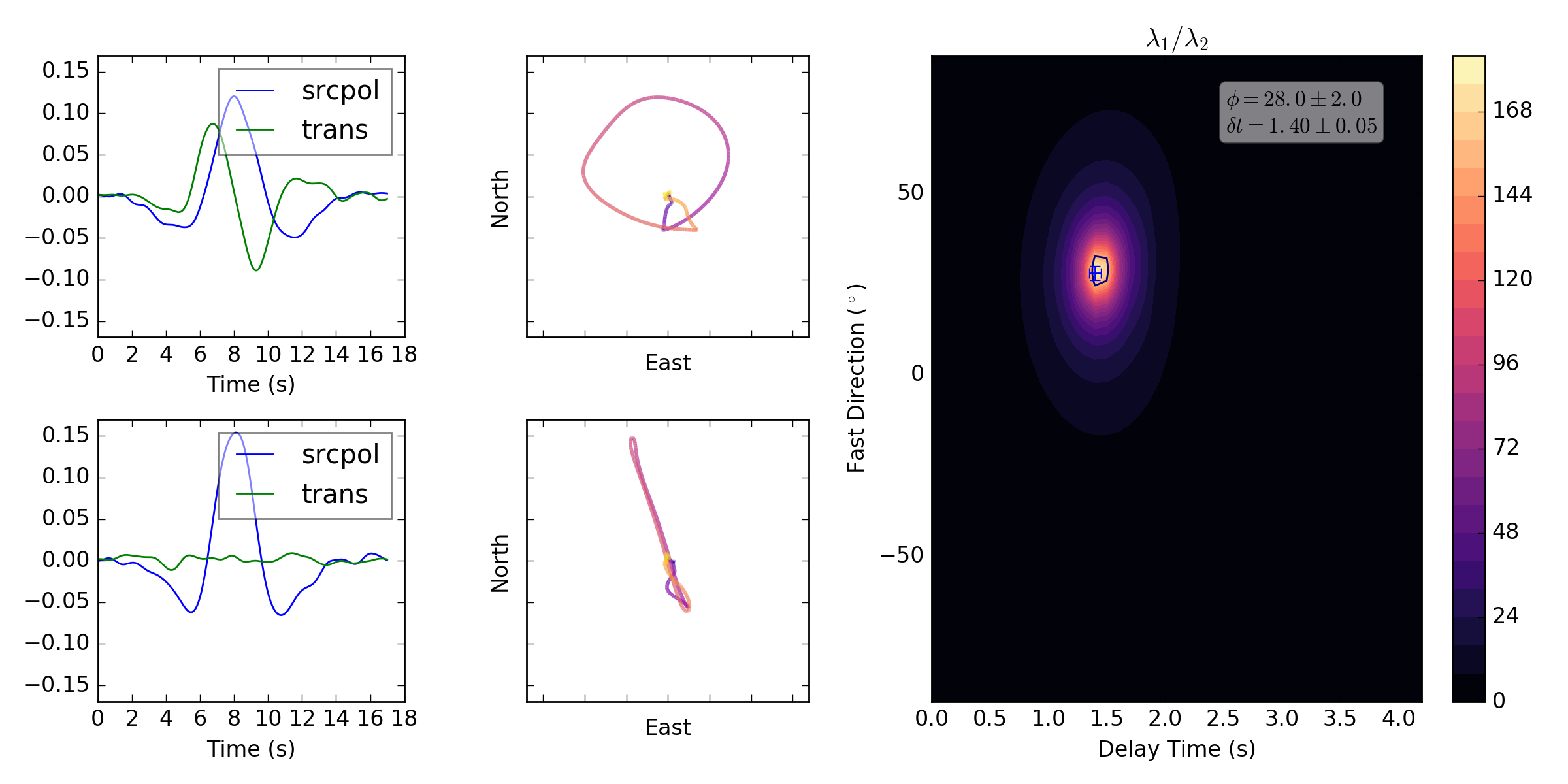
Silver and Chan (1991) eigenvalue method
A powerful and popular method for measuring splitting is the eigenvalue method of Silver and Chan (1991). It uses a grid search to find the inverse splitting parameters that best linearise the particle motion. Linearisation is assessed by principal component analysis at each search node, taking the eigenvalues of the covariance matrix, where linearity maximises \(\lambda_1\) and minimises \(\lambda_2\). The code uses the ratio \(\lambda_1/\lambda_2\) to find the best node (which is more stable than using only \(\lambda_1\) or \(\lambda_2\) as it accounts for the possibility that energy might be lost by sliding out of the window).
To use this method on your data.
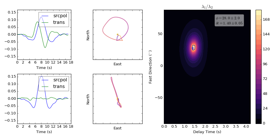
measure = sw.EigenM(data)
measure.plot()
Setting the lag time grid search
The code automatically sets the maximum lag time to be half the window length. To set the max search time manually you use the lags keyword. This accepts a tuple of length 1, 2, or 3, and will be interpreted differently depending on this length. The rules are as follows: for a 1-tuple lags = (maxlag,), a 2-tuple lags = (maxlag, nlags), and finally a 3-tuple (minlag, maxlag, nlags). Alternatively will accept a numpy array containing all nodes to search.
Setting the fast direction grid search
The code automatically grid searches every 2 degrees along the fast direction axis. That’s degs = 90 nodes in total (180/2). You can change this number using the degs keyword and providing an integer. Alternatively will accept a numpy array containing all nodes to search.
Saving and loading your measurements
To save your measurement to disk simply use the save(filename) method.
This will backup the input data complete with the \(\lambda_1\) and \(\lambda_2\) surfaces.
This can be recovered at a later time using splitwavepy.load(filename).
This feature is demonstrated here Get started.
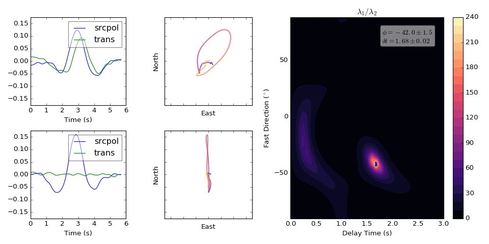
Splitting corrections
In the case where you have a good estimation of the splitting parameters beneath the receiver or the source it is possible to correct the waveforms and to measure the residual splitting. The residual splitting can then be attributed to anisotropy elsewhere along the path.
Let’s consider a simple 2-layer case.
# srcside and rceiver splitting parameters
srcsplit = (  30, 1.3)
rcvsplit = ( -44, 1.7)

# Create synthetic
a = sw.Pair( split=([ srcsplit, rcvsplit]), noise=0.03, delta=0.02)

# standard measurement
m = sw.EigenM(a, lags=(3,))
m.plot()
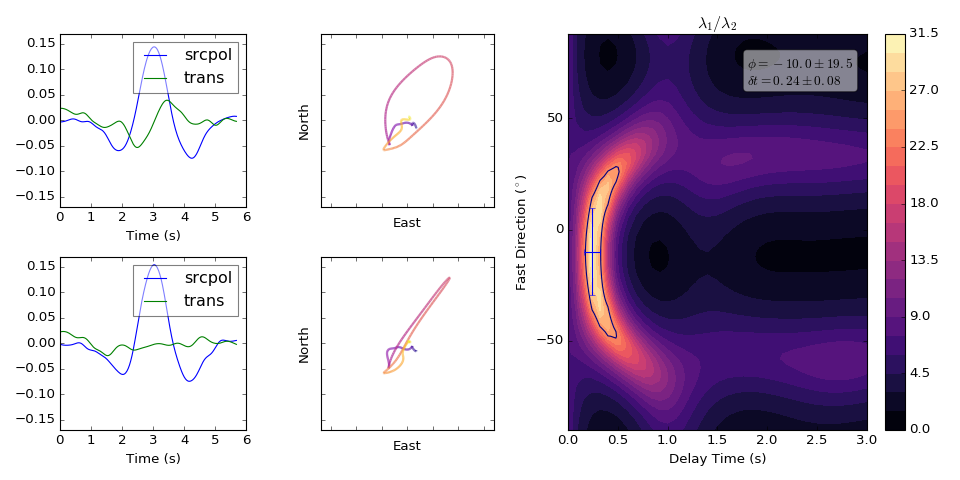
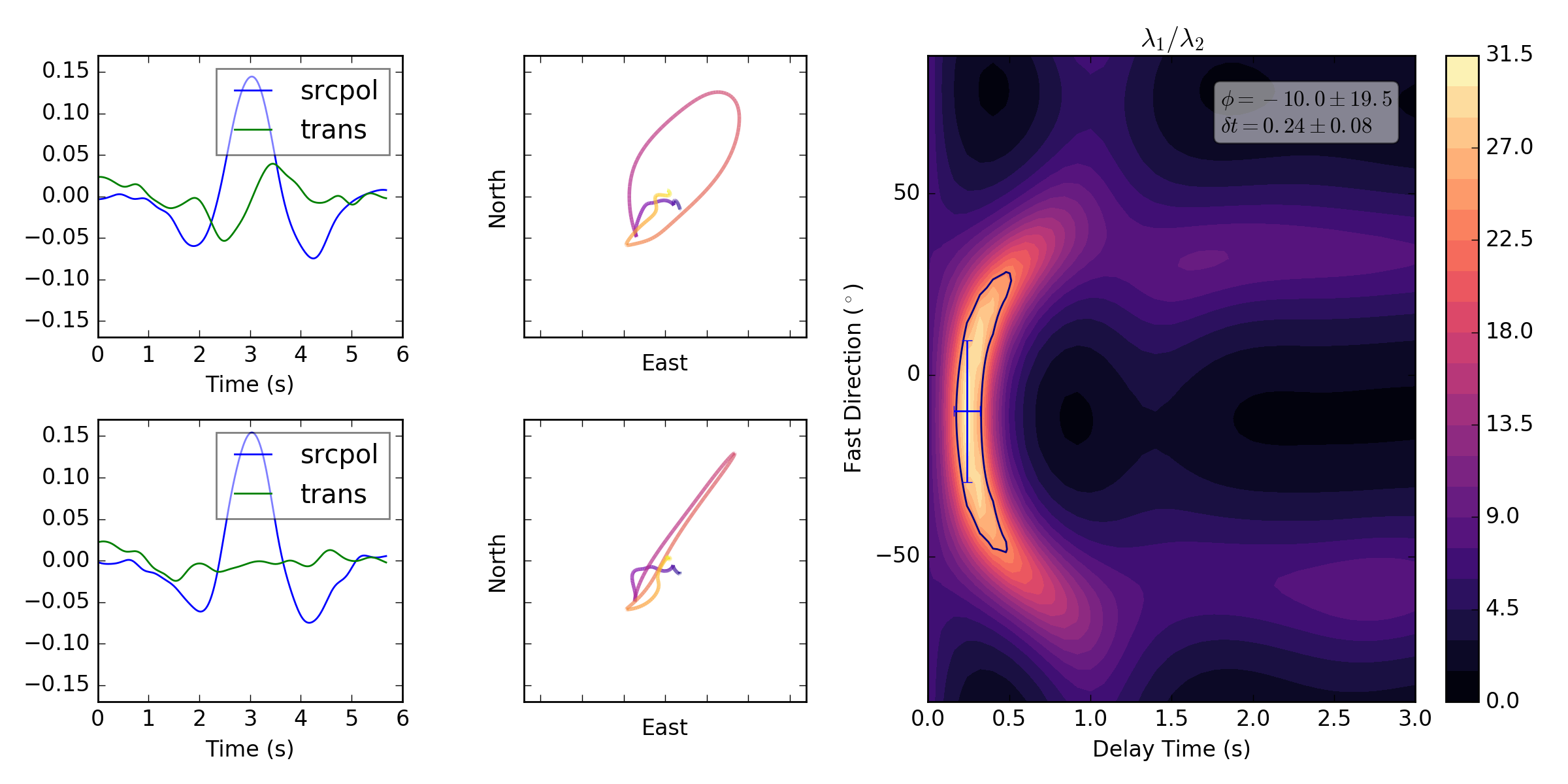

The apparent splitting measured above is some non-linear combination of the 2-layers (non-linear because the order of splitting is important).
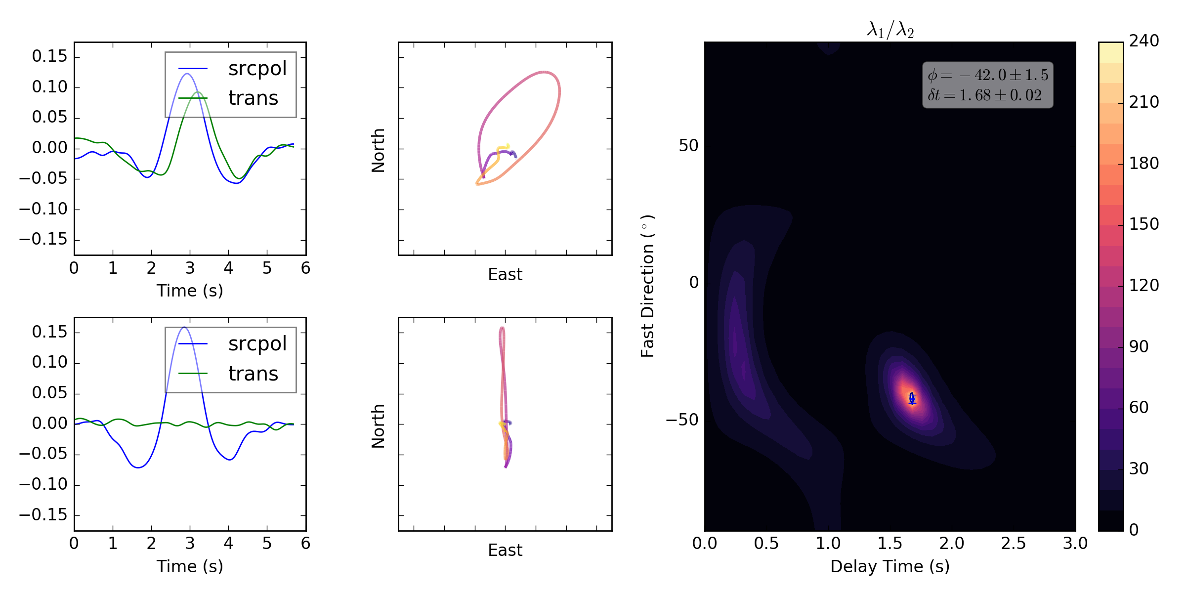
Receiver correction
If we know the layer 2 contribution we can back this off and resolve the splitting in layer 1 using the rcvcorr=(fast, lag) keyword.
m = sw.EigenM(a, lags=(3,), rcvcorr=(-44,1.7))
m.plot()
If it’s worked we should have measured splitting parameters of \(\phi=30\) and \(\delta t =1.3\).
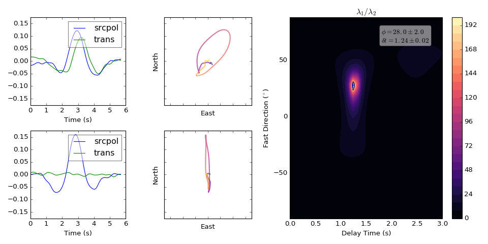
Source correction
Alternatively, if we know the layer 1 contribution we can use
srccorr=(fast, lag) to correct for the source side anisotropy.
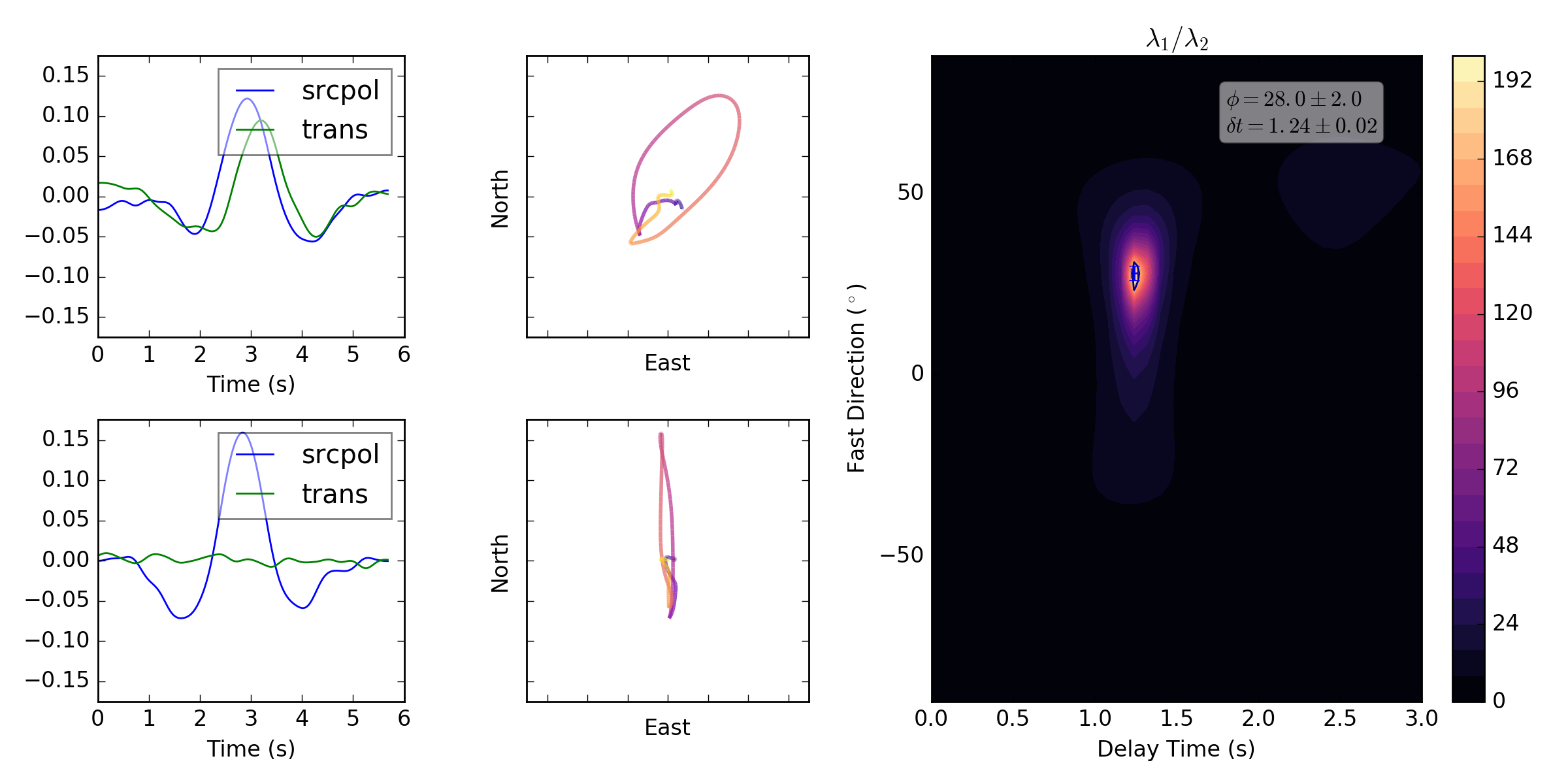
m = sw.EigenM(a, lags=(3,), srccorr=(30,1.3))
m.plot()
If this has worked we should have measured splitting parameters of \(\phi=-44\) and \(\delta t =1.7\).
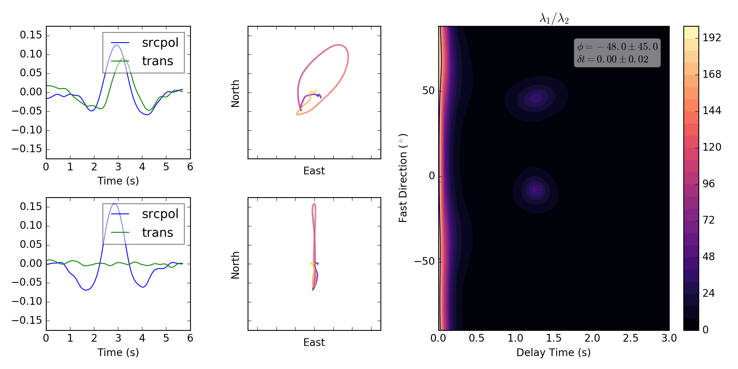
If we apply both the source and receiver correction to the above synthetic example we should yield a null result (no splitting).
m = sw.EigenM(a, lags=(3,), rcvcorr=(-44,1.7), srccorr=(30,1.3))
m.plot()
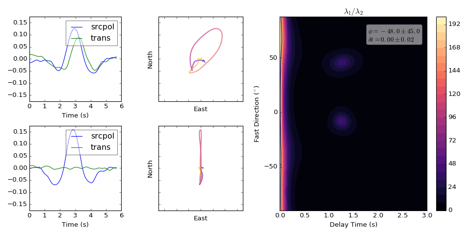
We do as can be seen by the concentration of energy at delay time 0.