Real data example

If you’ve got real data you need to get it into a numpy array. For the purposes of this tutorial, let’s use Obspy to download some data from the IRIS servers.

Preparing data

With real data it’s worth doing a bit of pre-processing which at minimum will involve removing the mean from data, and might also involve bandpass filtering, interpolation, and/or rotating the components. It is also necessary to pick the shear arrival of interest. All of this is achievable in Obspy.

from obspy import read
from obspy.clients.fdsn import Client
from obspy import UTCDateTime

client = Client("IRIS")
t = UTCDateTime("2000-08-15T04:30:0.000")
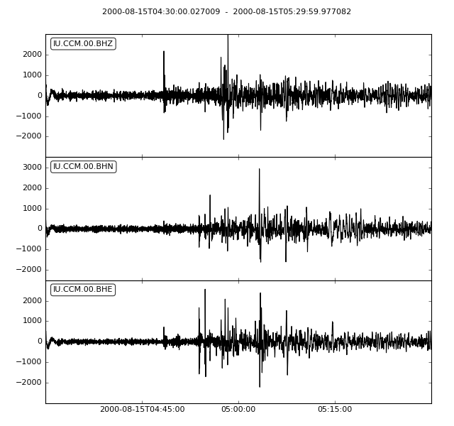
st = client.get_waveforms("IU", "CCM", "00", "BH?", t, t + 60 * 60,attach_response=True)

# filter the data (this process removes the mean)
st.filter("bandpass",freqmin=0.01,freqmax=0.5)

st.plot()

(png, hires.png, pdf)

When measuring splitting we need to have a specific shear wave arrival to target. Let’s use the obspy taup module to home in on the SKS arrival.

from obspy.taup import TauPyModel

# from location and time, get event information
lat=-31.56
lon=179.74

# server does not accept longitude greater than 180.
cat = client.get_events(starttime=t-60,endtime=t+60,minlatitude=lat-1,
                  maxlatitude=lat+1,minlongitude=lon-1,maxlongitude=180)
evtime = cat.events[0].origins[0].time
evdepth = cat.events[0].origins[0].depth/1000
evlat = cat.events[0].origins[0].latitude
evlon = cat.events[0].origins[0].longitude

# station information
inventory = client.get_stations(network="IU",station="CCM",starttime=t-60,endtime=t+60)
stlat = inventory[0][0].latitude
stlon = inventory[0][0].longitude

# find arrival times
model = TauPyModel('iasp91')
arrivals = model.get_travel_times_geo(evdepth,evlat,evlon,stlat,stlon,phase_list=['SKS'])
skstime = evtime + arrivals[0].time

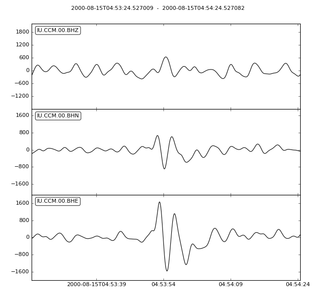
# trim around SKS
st.trim( skstime-30, skstime+30)
st.plot()

(png, hires.png, pdf)

Measuring splitting

Now we have prepared data we are ready to measure splitting.

First read the shear plane components (horizontals in this case) into a Pair object.

import splitwavepy as sw

# get data into Pair object and plot
north = st[1].data
east = st[0].data
sample_interval = st[0].stats.delta
realdata = sw.Pair(north, east, delta=sample_interval)
realdata.plot()

Note

Order is important. SplitWavePy expects the North component first.

By chance the window looks not bad. If you want to change it see Setting the window. For now let’s press on with measuring the splitting.

measure = sw.EigenM(realdata)
measure.plot()

It worked, kind of. The maximum delay time in the grid search is a bit high. We can change this using the lags keyword lags=(2,) as explained in Setting the lag time grid search.

measure = sw.EigenM(realdata, lags=(2,))
measure.plot()

Now see how to apply the Transverse Minimisation Method.